Persistent Homology Software: Demonstration of TDA
Demonstrating an open-source implementation of persistent homology techniques in the TDA package for R.
This post is part of the series The Data Scientist's Guide to Topological Data Analysis.
Want to get notified about new posts? Join the mailing list and follow on X/Twitter.
An R package named TDA (Fasy et al. 2014) has persistent homology capabilities, which we will demonstrate on another ND logo dataset.
n_x <- c(rep(-1,31),0.005*seq(-200,-50,5),rep(-.25,31))
n_y <- c(0.01*seq(-75,75,5),-0.01*seq(-75,75,5),
         0.01*seq(-75,75,5))

d_x <- c(rep(.25,31),
         0.15+sqrt(0.75^2-(0.01*seq(-75,75,5))^2))
d_y <- c(0.01*seq(-75,75,5),0.01*seq(-75,75,5))

nd <- data.frame(x=c(n_x,d_x),y=c(n_y,d_y))
plot(nd)
We’ll create a barcode diagram to display the dataset’s persistent homology in dimensions 0 and 1, for epsilon ranging from 0 to 1. The first homology components are colored black, while the second homology components are colored red.
Diag <- ripsDiag(X = nd, maxdimension = 2, maxscale = 1,
                 library = "GUDHI", printProgress = FALSE)
plot(Diag[["diagram"]], barcode = TRUE, main = "Barcode")
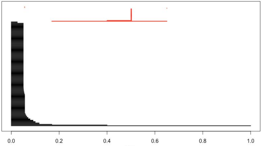
In first homology we see one component that persists the whole way, capturing the N and D together, and another component that persists about halfway, capturing the separation between the N and the D. In second homology, we see one component that persists halfway and captures the hole in the D.
Birth-death diagrams are also used to display the same information as persistence barcodes:
plot(Diag[["diagram"]])

There are also functions for calculating the Bottleneck and Wasserstein distances, which measure dissimilarity between homology diagrams. Below, we calculate these distances between the N and the D in the logo.
n <- data.frame(x = n_x, y = n_y)
d <- data.frame(x = d_x, y = d_y)

DiagN <- ripsDiag(X = n, maxdimension = 1, maxscale = 1)
DiagD <- ripsDiag(X = d, maxdimension = 1, maxscale = 1)

> print(bottleneck(Diag1 = DiagN[["diagram"]],
        Diag2 = DiagD[["diagram"]], dimension = 1))
0.2404992

> print(wasserstein(Diag1 = DiagN[["diagram"]],
        Diag2 = DiagD[["diagram"]], p = 2, dimension = 1))
0.05783988
References
- Fasy, Brittany, Jisu Kim, Fabrizio Lecci, Clement Maria, and Vincent Rouvreau. "Introduction to the R Package TDA." CRAN. 2014.
This post is part of the series The Data Scientist's Guide to Topological Data Analysis.
Want to get notified about new posts? Join the mailing list and follow on X/Twitter.