A Brief Overview of Spike-Timing Dependent Plasticity (STDP) Learning During Neural Simulation

by Justin Skycak on February 19, 2015

Implementation notes for STDP learning in a network of Hodgkin-Huxley simulated neurons.

Spike-Timing Dependent Plasticity (STDP) learning describes how neural connectivity changes depend on relative timing of neural spikes [2]. Specifically, when presynaptic and postsynaptic spikes are induced in neurons, resulting in presynaptic spikes at times $\lbrace t_{pre}^a \rbrace_{a \geq 1}$ and postsynaptic spikes at times $\lbrace t_{post}^b \rbrace_{b \geq 1},$ it is found [3] that the relative change in connection weight is given by

$\begin{align*} \frac{\Delta w_{post,pre}}{w_{post,pre}} = \sum_{a,b} \mathcal{W}(t_{post}^b - t_{pre}^a) \end{align*}$

where $\mathcal{W}$ is an STDP function. A choice of

$\begin{align*} \mathcal{W}(t) = \begin{cases} A_{+} \exp \lbrace - \frac{t}{\tau_+} \rbrace & t > 0 \\ A_{-} \exp \lbrace - \frac{t}{\tau_-} \rbrace & t < 0 \end{cases} \end{align*}$

with time constants $\tau_+, \tau_- \approx 10$ ms has been consistent empirical findings [4].

Implementation of STDP Learning

Consider a network of Hodgkin-Huxley [1] simulated neurons. Let $V_i(t)$ and $I_i(t)$ represent the voltage and current of the $i$th Hodgkin-Huxley neuron in a network. This neuron receives an external stimulus consisting of an electrode stimulus $s_i(t)$ and a stimulus $\sum\limits_{j \neq i} w_{ij}(t) I_j(t)$ from other neurons. The external stimulus adds to the current $I_i(t).$

Whenever $V_i(t)$ is updated, we check whether it is increasing and has crossed a threshold voltage $\phi = 60 \textrm{ mV}$ which we take to imply an action potential has occurred. If $V_i(t) < \phi < V_i(t + \Delta t),$ then we take $t + \Delta t$ to be a crossover time for neuron $i.$

For simplicity, we begin updating weights only after an amount of time equal to our update window $\ell$ has passed, and we stop updating weights $\ell$ steps before the end of simulation. After updating all the neurons in a given timestep, we look at the crossover times to determine the time differences in action potentials, and we use $\mathcal{W}(t)$ to adjust the weights accordingly.

Example and Interpretation of a 2-Neuron Simulation

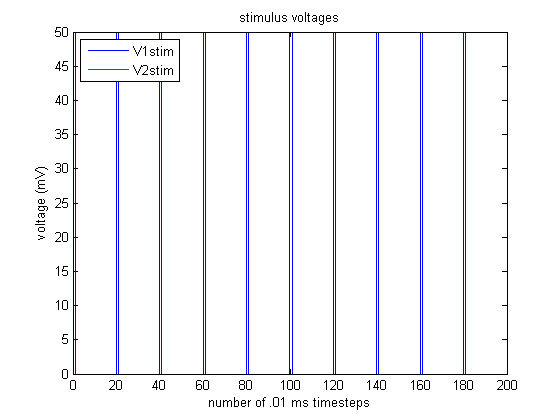
Here, we see an example trial. Neuron 1 is stimulated with a periodic 50 mV stimulus, as shown below:

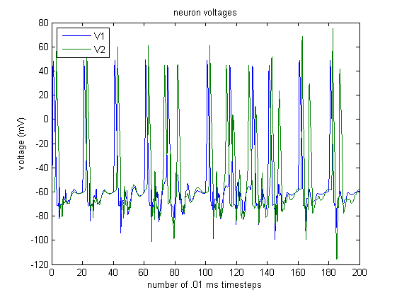
Assuming that the initial $1 \rightarrow 2$ and $2 \rightarrow 1$ connection weights are both 1, we observe the following activity:

Using the STDP scheme, the $1 \rightarrow 2$ and $2 \rightarrow 1$ synapse weights change as follows:

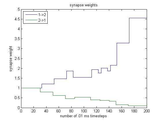
Explanation of Steps 0-40

The weights remain constant because the learning interval has not yet been reached.

Explanation of Steps 40-80

We see that for steps $\sim 40$ to $\sim 80,$ the weight of the $1 \rightarrow 2$ synapse increases. This makes sense because neuron 1 is being stimulated, neuron 1 excites neuron 2 with weight 2, and so stimulation in neuron 1 causes neuron 2 to spike quickly afterwards.

On the other hand, the weight of the $2 \rightarrow 1$ synapse is decreasing. Although spikes in neuron 2 excite neuron 1, they occur right after neuron 1 has spiked, so neuron 1 is in its refractory period and cannot spike. Thus, the $2 \rightarrow 1$ synapse weight decreases.

Explanation of Steps 80-140

During this period, the change in weight causes neuron 2 to become very eager to spike whenever $V_1$ increases sharply, and the $1 \rightarrow 2$ weight oscillates. We see that between steps $\sim 80$ and $\sim 140,$ a sharp increase in $V_1$ causes neuron 2 to spike. However, the sharp increase in $V_1$ does not lead into a spike in neuron 1, so the $1 \rightarrow 2$ weight decreases. However, neuron 2’s spike incites a spike in neuron 1, which incites another spike (of lesser magnitude) in neuron 2, so the $1 \rightarrow 2$ weight increases. This explains the $1 \rightarrow 2$ oscillation.

When neuron 2 spikes immediately prior to neuron 1, the $2 \rightarrow 1$ synapse increases. However, when neuron 2 spikes in response to a spike from neuron 1, the $2 \rightarrow 1$ synapse decreases. Overall, the $2 \rightarrow 1$ synapse remains roughly constant during this interval because its magnitude is so low.

Explanation of Steps 130-200

At these steps, the $1 \rightarrow 2$ synapse weight is so large that when neuron 1 spikes, it incites a spike in neuron 2, and when neuron 1 returns from hyperpolarization to resting state, neuron 2 spikes again. Because each spike in neuron 1 is followed by two spikes in neuron 2, the $1 \rightarrow 2$ weight increases greatly.

However, spikes in neuron 1 do not immediately follow spikes in neuron 2, so the $2 \rightarrow 1$ synapse weight becomes closer and closer to 0.

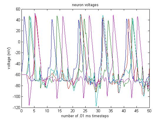
A 5-Neuron Simulation

References

[1] Hodgkin, A. L., \& Huxley, A. F. (1952). A quantitative description of membrane current and its application to conduction and excitation in nerve. The Journal of Physiology, 117(4), 500–544.

[2] Jesper Sjöström and Wulfram Gerstner (2010), Scholarpedia, 5(2):1362.

[3] Gerstner, W., Kempter R., van Hemmen J.L., and Wagner H. (1996). A neuronal learning rule for sub-millisecond temporal coding. Nature, 386:76-78.

[4] Zhang, L. I., Tao, H. W., Holt, C. E., Harris, W. A., and Poo, M.-M. (1998). A critical window for cooperation and competition among developing retinotectal synapses. Nature, 395:37-44.